Working with Percentiles (and Quantiles) of Distributions

Many times we want to observe different distributional properties of scenario data. The pyam function compute.quantiles() can help!

0. Define timeseries data and initialize an IamDataFrame

This tutorial uses a scenario similar to the data in the first-steps tutorial (here on GitHub and on read the docs).

Please read that tutorial for the reference and further information.

from pyam import IamDataFrame

df = IamDataFrame(data="tutorial_data.csv")
df.timeseries().head()

[INFO] 16:21:43 - pyam.core: Reading file tutorial_data.csv

					2010	2020	2030	2040	2050	2060	2070	2080	2090	2100
model	scenario	region	variable	unit
AIM/CGE 2.1	CD-LINKS_INDCi	R5ASIA	Emissions|CO2	Mt CO2/yr	11231.0880	14359.2801	14873.5967	15238.9081	15180.1854	15513.1760	16003.2060	16343.3124	17097.8681	17722.1245
			Primary Energy	EJ/yr	145.7409	191.0565	216.2135	234.2793	245.9771	258.3201	268.7644	275.0764	283.1479	288.6838
			Primary Energy|Biomass	EJ/yr	23.6647	24.0751	25.9262	27.3646	29.6938	29.8102	30.1178	30.0109	29.6166	29.5846
			Primary Energy|Fossil	EJ/yr	116.1932	155.0735	168.2376	179.0562	185.2168	195.6202	203.4916	207.3614	214.7828	217.7714
			Primary Energy|Non-Biomass Renewables	EJ/yr	4.5139	9.2641	17.0767	22.0967	25.3211	26.6589	27.9490	29.3259	29.3942	30.6799

1. Let’s see how many scenarios define CO2 emissions

df.filter(variable="Emissions|CO2", region="World").scenario

['1.0',
 'CD-LINKS_INDCi',
 'CD-LINKS_NPi',
 'CD-LINKS_NPi2020_1000',
 'CD-LINKS_NPi2020_1600',
 'CD-LINKS_NPi2020_400',
 'CD-LINKS_NoPolicy',
 'Faster Transition Scenario']

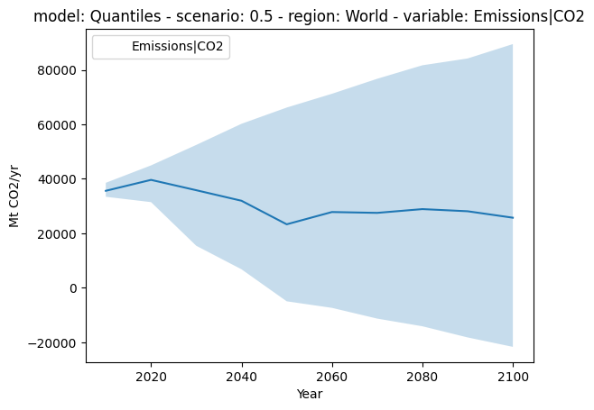
2. Get the median

The median is the 0.5 quantile (or percentile) - let’s take a look!

from matplotlib import pyplot as plt

fig, ax = plt.subplots()

# plot the background field of scenario data
(
    df.filter(variable="Emissions|CO2", region="World").plot.line(
        color="variable", alpha=0, fill_between=True, ax=ax
    )
)

# plot just the median
(
    df.filter(variable="Emissions|CO2", region="World")
    .compute.quantiles([0.5])
    .plot.line(ax=ax)
)

<Axes: title={'center': 'model: Quantiles - scenario: 0.5 - region: World - variable: Emissions|CO2'}, xlabel='Year', ylabel='Mt CO2/yr'>

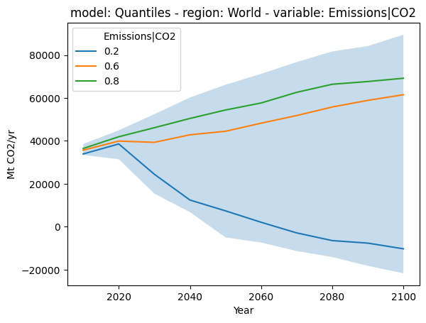
3. Get arbitrary quantiles

fig, ax = plt.subplots()

# plot the background field of scenario data
(
    df.filter(variable="Emissions|CO2", region="World").plot.line(
        color="variable", alpha=0, fill_between=True, ax=ax
    )
)

# plot quantiles
(
    df.filter(variable="Emissions|CO2", region="World")
    .compute.quantiles([0.2, 0.6, 0.8])
    .plot.line(ax=ax)
)

<Axes: title={'center': 'model: Quantiles - region: World - variable: Emissions|CO2'}, xlabel='Year', ylabel='Mt CO2/yr'>

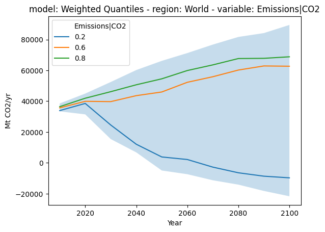
4. Weighted Quantiles

Weighted quantiles are also supported via the wquantiles package and are keyed to model/scenario combinations (unless the level argument is provided to compute.quantiles()).

import numpy as np

weights = df.meta.assign(weight=np.random.rand(len(df.meta)))
weights.head()

		weight
model	scenario
AIM/CGE 2.1	CD-LINKS_INDCi	0.890174
	CD-LINKS_NPi	0.077682
	CD-LINKS_NPi2020_1000	0.364202
	CD-LINKS_NPi2020_1600	0.305781
	CD-LINKS_NPi2020_400	0.191420

fig, ax = plt.subplots()

# plot the background field of scenario data
(
    df.filter(variable="Emissions|CO2", region="World").plot.line(
        color="variable", alpha=0, fill_between=True, ax=ax
    )
)

# plot weighted quantiles
(
    df.filter(variable="Emissions|CO2", region="World")
    .compute.quantiles([0.2, 0.6, 0.8], weights=weights["weight"])
    .plot.line(ax=ax)
)

<Axes: title={'center': 'model: Weighted Quantiles - region: World - variable: Emissions|CO2'}, xlabel='Year', ylabel='Mt CO2/yr'>