First steps with the pyam package

Scope and feature overview

The pyam package provides a range of diagnostic tools and functions for analyzing, visualizing and working with timeseries data following the format established by the Integrated Assessment Modeling Consortium (IAMC).

The format has been used in several IPCC assessments and numerous model comparison exercises. An illustrative example of this format template is shown below; read the docs for more information.

Model	Scenario	Region	Variable	Unit	2005	2010	2015
MESSAGE	CD-LINKS 400	World	Primary Energy	EJ/y	462.5	500.7	…

This notebook illustrates the basic functionality of the pyam package and the IamDataFrame class:

0. Load timeseries data from a snapshot file and inspect the scenario ensemble

1. Apply filters to the ensemble and display the timeseries data as pandas.DataFrame

2. Visualize timeseries data using the plotting library based on the matplotlib package

3. Perform scenario diagnostic and validation checks

4. Categorize scenarios according to timeseries data values

5. Compute quantitative indicators for further scenario characterization & diagnostics

6. Export data and categorization to a file

Read the docs

A comprehensive documentation is available at pyam-iamc.readthedocs.io.

Tutorial data

The timeseries data used in this tutorial is a partial snapshot of the scenario ensemble compiled for the IPCC’s Special Report on Global Warming of 1.5°C (SR15). The complete scenario ensemble data is publicly available from the IAMC 1.5°C Scenario Explorer and Data hosted by IIASA.

Please read the License page of the IAMC 1.5°C Scenario Explorer before using the full scenario data for scientific analysis or other work.

Scenarios in the tutorial data

The data used for this tutorial consists of selected variables from these sources:

• an ensemble of scenarios from the Horizon 2020 CD-LINKS project

• the “Faster Transition Scenario” from the IEA’s World Energy Outlook 2017,

• the “1.0” scenario submitted by the GENeSYS-MOD team (Löffler et al., 2017)

Please refer to the About page of the IAMC 1.5°C Scenario Explorer for references and additional information.

The data used here is a partial snapshot of the IAMC 1.5°C Scenario Data!

This tutorial is only intended as an illustration of the pyam package.

Citation of the scenario ensemble

D. Huppmann, E. Kriegler, V. Krey, K. Riahi, J. Rogelj, K. Calvin, F. Humpenoeder, A. Popp, S. K. Rose, J. Weyant, et al.

IAMC 1.5°C Scenario Explorer and Data hosted by IIASA (release 2.0)

Integrated Assessment Modeling Consortium & International Institute for Applied Systems Analysis, 2019.

doi: 10.5281/zenodo.3363345 | url: data.ece.iiasa.ac.at/iamc-1.5c-explorer

---

Import data from file and inspect the scenario

We import the snapshot of the timeseries data from the file tutorial_data.csv.

If you haven’t cloned the pyam GitHub repository to your machine, you can download the data file from the folder docs/tutorials.

Make sure to place the data file in the same folder as this notebook.

import pyam

df = pyam.IamDataFrame(data="tutorial_data.csv")

[INFO] 12:12:17 - pyam.core: Reading file tutorial_data.csv

/home/docs/checkouts/readthedocs.org/user_builds/pyam-iamc/checkouts/stable/pyam/utils.py:318: FutureWarning: The previous implementation of stack is deprecated and will be removed in a future version of pandas. See the What's New notes for pandas 2.1.0 for details. Specify future_stack=True to adopt the new implementation and silence this warning.
  .stack(dropna=True)

As a first step, we show an overview of the IamDataFrame content by simply calling df (alternatively, you can use print(df) or df.info()).

This function returns a concise (abbreviated) overview of the index dimensions and the qualitative/quantitative meta indicators (see an explanation of indicators below).

df

<class 'pyam.core.IamDataFrame'>
Index:
 * model    : AIM/CGE 2.1, GENeSYS-MOD 1.0, ... WITCH-GLOBIOM 4.4 (8)
 * scenario : 1.0, CD-LINKS_INDCi, CD-LINKS_NPi, ... Faster Transition Scenario (8)
Timeseries data coordinates:
   region   : R5ASIA, R5LAM, R5MAF, R5OECD90+EU, R5REF, R5ROWO, World (7)
   variable : ... (6)
   unit     : EJ/yr, Mt CO2/yr, °C (3)
   year     : 2010, 2020, 2030, 2040, 2050, 2060, 2070, 2080, ... 2100 (10)

In the following cells, we display the lists of all models, scenarios, regions, and the mapping of variables to units in the snapshot.

df.model

['AIM/CGE 2.1',
 'GENeSYS-MOD 1.0',
 'IEA World Energy Model 2017',
 'IMAGE 3.0.1',
 'MESSAGEix-GLOBIOM 1.0',
 'POLES CD-LINKS',
 'REMIND-MAgPIE 1.7-3.0',
 'WITCH-GLOBIOM 4.4']

df.scenario

['1.0',
 'CD-LINKS_INDCi',
 'CD-LINKS_NPi',
 'CD-LINKS_NPi2020_1000',
 'CD-LINKS_NPi2020_1600',
 'CD-LINKS_NPi2020_400',
 'CD-LINKS_NoPolicy',
 'Faster Transition Scenario']

df.region

['R5ASIA', 'R5LAM', 'R5MAF', 'R5OECD90+EU', 'R5REF', 'R5ROWO', 'World']

df.unit_mapping

{'AR5 climate diagnostics|Temperature|Global Mean|MAGICC6|MED': '°C',
 'Emissions|CO2': 'Mt CO2/yr',
 'Primary Energy': 'EJ/yr',
 'Primary Energy|Biomass': 'EJ/yr',
 'Primary Energy|Fossil': 'EJ/yr',
 'Primary Energy|Non-Biomass Renewables': 'EJ/yr'}

Apply filters to the ensemble and display the timeseries data

A selection of the timeseries data of an IamDataFrame can be obtained by applying the filter() function, which takes keyword-arguments of criteria. The function returns a down-selected clone of the IamDataFrame instance.

Filtering by model names, scenarios and regions

The feature for filtering by model, scenario or region are implemented using exact string matching, where * can be used as a wildcard.

First, we want to display the list of all scenarios submitted by the MESSAGE modeling team.

Applying the filter argument model='MESSAGE' will return an empty array

(because the MESSAGE model in the tutorial data is actually called MESSAGEix-GLOBIOM 1.0)

df.filter(model="MESSAGE").scenario

[WARNING] 12:12:17 - pyam.core: Filtered IamDataFrame is empty!

[]

Filtering for model='MESSAGE*' will return all scenarios provided by the MESSAGEix-GLOBIOM 1.0 model

df.filter(model="MESSAGE*").scenario

['CD-LINKS_INDCi',
 'CD-LINKS_NPi',
 'CD-LINKS_NPi2020_1000',
 'CD-LINKS_NPi2020_1600',
 'CD-LINKS_NPi2020_400',
 'CD-LINKS_NoPolicy']

Inverting the selection

Using the keyword keep=False allows you to select the inverse of the filter arguments.

df.filter(region="World").region

['World']

df.filter(region="World", keep=False).region

['R5ASIA', 'R5LAM', 'R5MAF', 'R5OECD90+EU', 'R5REF', 'R5ROWO']

Filtering by variables and levels

Filtering for variable strings works in an identical way as above, with * available as a wildcard.

Filtering for Primary Energy will return only exactly those data

Filtering for Primary Energy|* will return all sub-categories of primary energy (and only the sub-categories)

In addition, variables can be filtered by their level, i.e., the “depth” of the variable in a hierarchical reading of the string separated by | (pipe, not L or i). That is, the variable Primary Energy has level 0, while Primary Energy|Fossil has level 1.

Filtering by both variables and level will search for the hierarchical depth following the variable string so filter arguments variable='Primary Energy*' and level=1 will return all variables immediately below Primary Energy. Filtering by level only will return all variables at that depth.

df.filter(variable="Primary Energy*", level=1).variable

['Primary Energy|Biomass',
 'Primary Energy|Fossil',
 'Primary Energy|Non-Biomass Renewables']

The next cell illustrates another use case of the level filter argument - filtering by 1- (as string) instead of 1 (as integer) will return all timeseries data for variables up to the specified depth.

df.filter(variable="Primary Energy*", level="1-").variable

['Primary Energy',
 'Primary Energy|Biomass',
 'Primary Energy|Fossil',
 'Primary Energy|Non-Biomass Renewables']

The last cell shows how to filter only by level without providing a variable argument. The example returns all variables that are at the second hierarchical level (i.e., not Primary Energy).

df.filter(level=1).variable

['Emissions|CO2',
 'Primary Energy|Biomass',
 'Primary Energy|Fossil',
 'Primary Energy|Non-Biomass Renewables']

Displaying timeseries data

As a next step, we want to view a selection of the timeseries data.

The timeseries() function returns the data as a pandas.DataFrame in the standard IAMC template.

This is a wide format table where years are shown as columns.

display_df = df.filter(model="MESSAGE*", variable="Primary Energy", region="World")
display_df.timeseries()

					2010	2020	2030	2040	2050	2060	2070	2080	2090	2100
model	scenario	region	variable	unit
MESSAGEix-GLOBIOM 1.0	CD-LINKS_INDCi	World	Primary Energy	EJ/yr	500.739995	550.751899	613.016704	699.467451	787.902841	864.193441	941.505687	1042.178884	1147.485190	1260.198089
	CD-LINKS_NPi	World	Primary Energy	EJ/yr	500.739995	550.751899	636.789216	719.268869	809.826701	883.520127	968.547117	1068.128998	1177.947712	1284.782597
	CD-LINKS_NPi2020_1000	World	Primary Energy	EJ/yr	500.739995	550.751899	572.210786	597.264498	658.349228	732.402145	803.457281	856.135227	902.853711	956.724237
	CD-LINKS_NPi2020_1600	World	Primary Energy	EJ/yr	500.739995	550.751899	602.620029	644.564918	683.285941	752.111932	835.886959	900.782509	955.826758	1010.768413
	CD-LINKS_NPi2020_400	World	Primary Energy	EJ/yr	500.739995	550.751899	518.026936	531.989826	594.736488	658.582662	717.555078	769.173895	823.638025	882.550952
	CD-LINKS_NoPolicy	World	Primary Energy	EJ/yr	500.739995	571.736041	651.554386	733.474469	828.476616	904.461233	986.679077	1089.824029	1201.254614	1306.794566

Filtering by year

Filtering for years can be done by one integer value, a list of integers, or the Python class range.

The last year of a range is not included, so range(2010, 2015) is interpreted as [2010, 2011, 2012, 2013, 2014].

The next cell shows the same down-selected IamDataFrame as above, but further reduced to three timesteps.

display_df.filter(year=[2010, 2030, 2050]).timeseries()

					2010	2030	2050
model	scenario	region	variable	unit
MESSAGEix-GLOBIOM 1.0	CD-LINKS_INDCi	World	Primary Energy	EJ/yr	500.739995	613.016704	787.902841
	CD-LINKS_NPi	World	Primary Energy	EJ/yr	500.739995	636.789216	809.826701
	CD-LINKS_NPi2020_1000	World	Primary Energy	EJ/yr	500.739995	572.210786	658.349228
	CD-LINKS_NPi2020_1600	World	Primary Energy	EJ/yr	500.739995	602.620029	683.285941
	CD-LINKS_NPi2020_400	World	Primary Energy	EJ/yr	500.739995	518.026936	594.736488
	CD-LINKS_NoPolicy	World	Primary Energy	EJ/yr	500.739995	651.554386	828.476616

Parallels to the pandas data analysis toolkit

When developing pyam, we followed the syntax of the Python package pandas (read the docs) closely where possible. In many cases, you can use similar functions directly on the IamDataFrame.

In the next cell, we illustrate this parallel behaviour. The function pyam.IamDataFrame.head() is similar to pandas.DataFrame.head(): it returns the first n rows of the ‘data’ table in long format (columns are in year/value format).

Similar to the timeseries() function shown above, the returned object of head() is a pandas.DataFrame.

display_df.head()

	model	scenario	region	variable	unit	year	value
0	MESSAGEix-GLOBIOM 1.0	CD-LINKS_INDCi	World	Primary Energy	EJ/yr	2010	500.739995
1	MESSAGEix-GLOBIOM 1.0	CD-LINKS_INDCi	World	Primary Energy	EJ/yr	2020	550.751899
2	MESSAGEix-GLOBIOM 1.0	CD-LINKS_INDCi	World	Primary Energy	EJ/yr	2030	613.016704
3	MESSAGEix-GLOBIOM 1.0	CD-LINKS_INDCi	World	Primary Energy	EJ/yr	2040	699.467451
4	MESSAGEix-GLOBIOM 1.0	CD-LINKS_INDCi	World	Primary Energy	EJ/yr	2050	787.902841

Getting help

When in doubt, you can look at the help for any function by appending a ?.

df.filter?

Visualize timeseries data using the plotting library

This section provides an illustrative example of the plotting features of the pyam package.

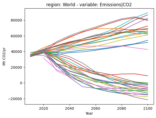
In the next cell, we show a simple line plot of global CO2 emissions. The colours are assigned randomly by default, and pyam deactivates the legend if there are too many lines.

df.filter(variable="Emissions|CO2", region="World").plot()

[INFO] 12:12:18 - pyam.plotting: >=13 labels, not applying legend

<Axes: title={'center': 'region: World - variable: Emissions|CO2'}, xlabel='Year', ylabel='Mt CO2/yr'>

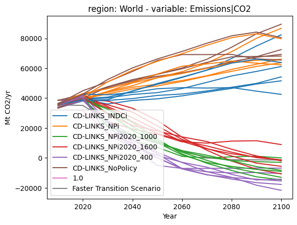
Most functions of the plotting library also take some intuitive keyword arguments for better styling options or using the same colors across groups of scenarios. For example, color='scenario' will use consistent colors for each scenario name (most of them implemented by multiple modeling frameworks). There are now less than 13 colors used, so the legend will be shown by default.

df.filter(variable="Emissions|CO2", region="World").plot(color="scenario")

<Axes: title={'center': 'region: World - variable: Emissions|CO2'}, xlabel='Year', ylabel='Mt CO2/yr'>

The section on categorization will show more options of the plotting features, as well as a method to set specific colors for different categories. For more information, look at the other tutorials and the plotting gallery.

Perform scenario diagnostic and validation checks

When analyzing scenario results, it is often useful to check whether certain timeseries data exist or the values are within a specific range. For example, it may make sense to ensure that reported data for historical periods are close to established reference data or that near-term developments are reasonable.

Before diving into the diagnostics and validation features, we need to briefly introduce the meta attribute. This attribute of an IamDataFrame is a pandas.DataFrame, which can be used to store categorization information and quantitative indicators of each model-scenario. In addition, an IamDataFrame has an attribubte exclude, which is a pandas.Series set to False for all model-scenario combinations.

The next cell shows the first 10 rows of the ‘meta’ table.

df.meta.head(10)

model	scenario
AIM/CGE 2.1	CD-LINKS_INDCi
	CD-LINKS_NPi
	CD-LINKS_NPi2020_1000
	CD-LINKS_NPi2020_1600
	CD-LINKS_NPi2020_400
	CD-LINKS_NoPolicy
GENeSYS-MOD 1.0	1.0
IEA World Energy Model 2017	Faster Transition Scenario
IMAGE 3.0.1	CD-LINKS_INDCi
	CD-LINKS_NPi

The following section provides three illustrations of the diagnostic tools: 0. Verify that a timeseries Primary Energy exists in each scenario (in at least one year and, in a second step, in the last year of the horizon). 1. Validate whether scenarios deviate by more than 10% from the Primary Energy reference data reported in the IEA Energy Statistics in 2010. 2. Use the exclude_on_fail option of the validation function to create a sub-selection of the scenario ensemble.

For simplicity, the example in this section operates on a down-selected data ensemble that only contains global values.

df_world = df.filter(region="World")

Check for required variables

We first use the require_data() function to assert that the scenarios contain data for the expected timeseries.

This method returns the list of scenarios and data rows where any combination of the required arguments are missing.

If the method returns None, all required data are present.

df_world.require_data(variable="Primary Energy")

df_world.require_data(variable="Primary Energy", year=2100)

	model	scenario	variable	year
0	GENeSYS-MOD 1.0	1.0	Primary Energy	2100
1	IEA World Energy Model 2017	Faster Transition Scenario	Primary Energy	2100

The two cells above show that all scenarios report primary-energy data, but not all scenarios provide this timeseries until the end of the century.

Validate numerical values in the timeseries data

The validate() function performs checks on specific values of timeseries data. The criteria argument specifies a valid range by an upper and lower bound (up, lo) for a variable and a subset of years to which the validation is applied - all scenarios with a value in at least one year outside that range are considered to not satisfy the validation. The function returns a list of data points not satisfying the criteria.

According to the IEA Energy Statistics, Total Primary Energy Supply was ~540 EJ in 2010. In the next cell, we show all data points that deviate (downwards) by more than 10% from this reference value.

df_world.validate(variable="Primary Energy", year=2010, lower_bound=540 * 0.9)

[INFO] 12:12:19 - pyam.validation: 6 of 2220 data points do not satisfy the criteria

	model	scenario	region	variable	unit	year	value
0	REMIND-MAgPIE 1.7-3.0	CD-LINKS_INDCi	World	Primary Energy	EJ/yr	2010	478.4152
1	REMIND-MAgPIE 1.7-3.0	CD-LINKS_NPi	World	Primary Energy	EJ/yr	2010	478.4152
2	REMIND-MAgPIE 1.7-3.0	CD-LINKS_NPi2020_1000	World	Primary Energy	EJ/yr	2010	478.4152
3	REMIND-MAgPIE 1.7-3.0	CD-LINKS_NPi2020_1600	World	Primary Energy	EJ/yr	2010	478.4152
4	REMIND-MAgPIE 1.7-3.0	CD-LINKS_NPi2020_400	World	Primary Energy	EJ/yr	2010	478.4152
5	REMIND-MAgPIE 1.7-3.0	CD-LINKS_NoPolicy	World	Primary Energy	EJ/yr	2010	478.4152

Use the exclude_on_fail feature to create a sub-selection of the scenario ensemble

Per default, the functions above only report how many scenarios or which data points do not satisfy the validation criteria above. However, they also have an option to exclude_on_fail, which marks all scenarios failing the validation as exclude=True in the ‘meta’ table. This feature can be particularly helpful when a user wants to perform a number of validation steps and then efficiently remove all scenarios violating any of the criteria as part of a scripted workflow.

We illustrate a simple validation workflow using the CO2 emissions. The next cell shows the trajectories of CO2 emissions across all scenarios.

df_world.filter(variable="Emissions|CO2").plot()

[INFO] 12:12:19 - pyam.plotting: >=13 labels, not applying legend

<Axes: title={'center': 'region: World - variable: Emissions|CO2'}, xlabel='Year', ylabel='Mt CO2/yr'>

The next two cells perform validation to exclude all scenarios that have implausibly low emissions in 2020 (i.e., unrealistic near-term behaviour) as well as those that do not reduce emissions over the century (i.e., exceed a value of 45000 MT CO2 in any year).

df_world.validate(
    variable="Emissions|CO2", year=2020, lower_bound=38000, exclude_on_fail=True
)

[INFO] 12:12:19 - pyam.validation: 2 of 2220 data points do not satisfy the criteria

[INFO] 12:12:19 - pyam.validation: 2 scenarios failed validation and will be set as `exclude=True`.

	model	scenario	region	variable	unit	year	value
0	GENeSYS-MOD 1.0	1.0	World	Emissions|CO2	Mt CO2/yr	2020	31449.00000
1	IEA World Energy Model 2017	Faster Transition Scenario	World	Emissions|CO2	Mt CO2/yr	2020	35128.48356

df_world.validate(variable="Emissions|CO2", upper_bound=45000, exclude_on_fail=True)

[INFO] 12:12:19 - pyam.validation: 119 of 2220 data points do not satisfy the criteria

[INFO] 12:12:19 - pyam.validation: 18 scenarios failed validation and will be set as `exclude=True`.

	model	scenario	region	variable	unit	year	value
0	AIM/CGE 2.1	CD-LINKS_INDCi	World	Emissions|CO2	Mt CO2/yr	2080	46515.03230
1	AIM/CGE 2.1	CD-LINKS_INDCi	World	Emissions|CO2	Mt CO2/yr	2090	49433.62680
2	AIM/CGE 2.1	CD-LINKS_INDCi	World	Emissions|CO2	Mt CO2/yr	2100	51588.30740
3	AIM/CGE 2.1	CD-LINKS_NPi	World	Emissions|CO2	Mt CO2/yr	2040	46122.39910
4	AIM/CGE 2.1	CD-LINKS_NPi	World	Emissions|CO2	Mt CO2/yr	2050	48146.98730
...	...	...	...	...	...	...	...
114	WITCH-GLOBIOM 4.4	CD-LINKS_NoPolicy	World	Emissions|CO2	Mt CO2/yr	2060	71218.41287
115	WITCH-GLOBIOM 4.4	CD-LINKS_NoPolicy	World	Emissions|CO2	Mt CO2/yr	2070	76719.27197
116	WITCH-GLOBIOM 4.4	CD-LINKS_NoPolicy	World	Emissions|CO2	Mt CO2/yr	2080	81678.20906
117	WITCH-GLOBIOM 4.4	CD-LINKS_NoPolicy	World	Emissions|CO2	Mt CO2/yr	2090	84177.35881
118	WITCH-GLOBIOM 4.4	CD-LINKS_NoPolicy	World	Emissions|CO2	Mt CO2/yr	2100	80467.95669

119 rows × 7 columns

We can select all scenarios that have not been marked to be excluded by adding exclude=False to the filter() statement.

To highlight the difference between the full scenario set and the reduced scenario set based on the validation exclusions, the next cell puts the two plots side by side with a shared y-axis.

import matplotlib.pyplot as plt

fig, ax = plt.subplots(1, 2, figsize=(8, 4), sharey=True)

df_world_co2 = df_world.filter(variable="Emissions|CO2")

df_world_co2.plot(ax=ax[0])
df_world_co2.filter(exclude=False).plot(ax=ax[1])

[INFO] 12:12:20 - pyam.plotting: >=13 labels, not applying legend

[INFO] 12:12:20 - pyam.plotting: >=13 labels, not applying legend

<Axes: title={'center': 'region: World - variable: Emissions|CO2'}, xlabel='Year', ylabel='Mt CO2/yr'>

Categorize scenarios according to timeseries data values

It is often useful to apply categorization to classes of scenarios according to specific characteristics of the timeseries data. In the following example, we use the median global mean temperature assessment (computed using MAGICC 6 in the AR5 configuration) to categorize scenarios by their warming by the end of the century (year 2100).

Cleaning up a scenario ensemble for simpler processing

When displaying the list of variables in the scenario ensemble earlier, you probably noticed that the variable for the temperature assessment had a rather unwieldy name: AR5 climate diagnostics|Temperature|Global Mean|MAGICC6|MED.

To simplify further processing, we use the rename() function to change the variable of this timeseries data to Temperature. By adding the argument inplace=True, the renaming is performed directly on the IamDataFrame rather than returning a copy with the change.

df.rename(
    variable={
        "AR5 climate diagnostics|Temperature|Global Mean|MAGICC6|MED": "Temperature"
    },
    inplace=True,
)

In the next cell, we display the list of variables again to verify that the renaming was successful.

df.variable

['Emissions|CO2',
 'Primary Energy',
 'Primary Energy|Biomass',
 'Primary Energy|Fossil',
 'Primary Energy|Non-Biomass Renewables',
 'Temperature']

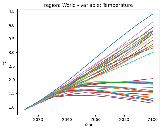
Now, we display the timeseries data of the warming outcome as a line plot. This helps to decide where to set the thresholds for the categories.

df.filter(variable="Temperature").plot()

[INFO] 12:12:20 - pyam.plotting: >=13 labels, not applying legend

<Axes: title={'center': 'region: World - variable: Temperature'}, xlabel='Year', ylabel='°C'>

Categorization assignment

We now use the categorization feature to group scenarios by their temperature outcome by the end of the century.

The first cell sets the Temperature categorization to the default ‘uncategorized’. This is not necessary per se (setting a meta column via the categorization will mark all non-assigned rows as ‘uncategorized’ (if the value is a string) or np.nan. However, having this cell may be helpful in this tutorial notebook if you are going back and forth between cells to reset the assignment.

The function categorize() takes color and similar arguments, which can then be used by the plotting library.

df.set_meta(meta="uncategorized", name="warming-category")

df.categorize(
    "warming-category",
    "below 1.6C",
    criteria={"Temperature": {"up": 1.6, "year": 2100}},
    color="xkcd:baby blue",
)

/home/docs/checkouts/readthedocs.org/user_builds/pyam-iamc/checkouts/stable/pyam/core.py:1111: DeprecationWarning: Argument `criteria` is deprecated and will be removed in future versions. Use `upper_bound`, `lower_bound`, and filter-arguments instead.
  return _validate(
[INFO] 12:12:21 - pyam.validation: 26 of 9940 data points do not satisfy the criteria

[INFO] 12:12:21 - pyam.core: 12 scenarios categorized as `warming-category: below 1.6C`

df.categorize(
    "warming-category",
    "below 2.5C",
    criteria={"Temperature": {"up": 2.5, "lo": 1.6, "year": 2100}},
    color="xkcd:green",
)

/home/docs/checkouts/readthedocs.org/user_builds/pyam-iamc/checkouts/stable/pyam/core.py:1111: DeprecationWarning: Argument `criteria` is deprecated and will be removed in future versions. Use `upper_bound`, `lower_bound`, and filter-arguments instead.
  return _validate(
[INFO] 12:12:21 - pyam.validation: 29 of 9940 data points do not satisfy the criteria

[INFO] 12:12:21 - pyam.core: 9 scenarios categorized as `warming-category: below 2.5C`

df.categorize(
    "warming-category",
    "below 3.5C",
    criteria={"Temperature": {"up": 3.5, "lo": 2.5, "year": 2100}},
    color="xkcd:goldenrod",
)

/home/docs/checkouts/readthedocs.org/user_builds/pyam-iamc/checkouts/stable/pyam/core.py:1111: DeprecationWarning: Argument `criteria` is deprecated and will be removed in future versions. Use `upper_bound`, `lower_bound`, and filter-arguments instead.
  return _validate(
[INFO] 12:12:21 - pyam.validation: 31 of 9940 data points do not satisfy the criteria

[INFO] 12:12:21 - pyam.core: 7 scenarios categorized as `warming-category: below 3.5C`

df.categorize(
    "warming-category",
    "above 3.5C",
    criteria={"Temperature": {"lo": 3.5, "year": 2100}},
    color="xkcd:crimson",
)

/home/docs/checkouts/readthedocs.org/user_builds/pyam-iamc/checkouts/stable/pyam/core.py:1111: DeprecationWarning: Argument `criteria` is deprecated and will be removed in future versions. Use `upper_bound`, `lower_bound`, and filter-arguments instead.
  return _validate(
[INFO] 12:12:21 - pyam.validation: 25 of 9940 data points do not satisfy the criteria

[INFO] 12:12:21 - pyam.core: 13 scenarios categorized as `warming-category: above 3.5C`

Apply categories to timeseries analysis

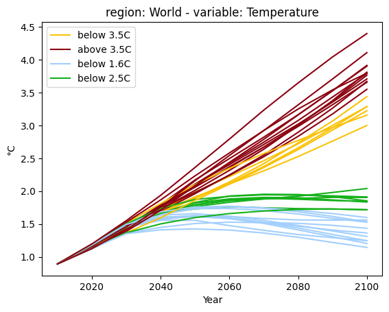
Now, we again display the median global temperature increase for all scenarios, but we use the colouring by category to illustrate the common characteristics across scenarios.

df.filter(variable="Temperature").plot(color="warming-category")

<Axes: title={'center': 'region: World - variable: Temperature'}, xlabel='Year', ylabel='°C'>

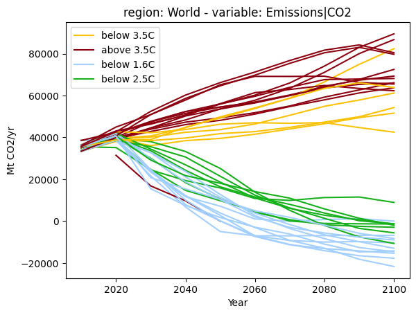
As a last step, we display the aggregate CO2 emissions, but apply the color scheme of the categorization by temperature. This allows to highlight alternative pathways within the same category.

Note that the emissions plot also includes one uncategorized scenario. The GENeSYS-MOD scenario did not provide timeseries data until the end of the century and hence could not be assessed for its warming outcome with MAGICC6 in the SR15 process.

df.filter(variable="Emissions|CO2", region="World").plot(color="warming-category")

<Axes: title={'center': 'region: World - variable: Emissions|CO2'}, xlabel='Year', ylabel='Mt CO2/yr'>

Compute quantitative indicators for further scenario characterization & diagnostics

In the previous section, we classified scenarios in distinct groups by their end-of-century warming outcome. In other use cases, however, it may be of interest to easily derive quantitative indicators and use those for more detailed scenario assessment.

In this section, we illustrate two ways to add quantitative indicators. First, we add two indicators derived directly from timeseries data: the warming at the end of the century (end-of-century-temperature) and the peak temperature over the entire model horizon (peak-temperature). For the end-of-century indicator, we can pass the year of relevant as a filter argument to the set_meta_from_data() function.

eoc = "end-of-century-temperature"
df.set_meta_from_data(name=eoc, variable="Temperature", year=2100)

If the filter arguments passed to set_meta_from_data() do not yield a unique value (in this case without a specific year), we can pass a method to aggregate or select a specific value (e.g., the maximum using the numpy package - read the docs).

import numpy as np

peak = "peak-temperature"
df.set_meta_from_data(name=peak, variable="Temperature", method=np.max)

The second method to define quantitative indicators is the function set_meta(). It can take any pandas.Series with an index including model and scenario.

In the example, we can now easily derive the “overshoot”, i.e., the reduction in global temperature after the peak, by computing the difference between the two quantitative indicators.

overshoot = df.meta[peak] - df.meta[eoc]
overshoot.head()

model        scenario
AIM/CGE 2.1  CD-LINKS_INDCi           0.000000
             CD-LINKS_NPi             0.000000
             CD-LINKS_NPi2020_1000    0.057239
             CD-LINKS_NPi2020_1600    0.000000
             CD-LINKS_NPi2020_400     0.310221
dtype: float64

df.set_meta(name="overshoot", meta=overshoot)

As a last step of this illustrative example, we again display the first 10 rows of the meta attribute of the IamDataFrame. The meta column seen in cell 20 now includes columns with the three quantitative indicators.

df.meta.head(10)

		warming-category	end-of-century-temperature	peak-temperature	overshoot
model	scenario
AIM/CGE 2.1	CD-LINKS_INDCi	below 3.5C	3.284531	3.284531	0.000000
	CD-LINKS_NPi	above 3.5C	3.707443	3.707443	0.000000
	CD-LINKS_NPi2020_1000	below 1.6C	1.560135	1.617375	0.057239
	CD-LINKS_NPi2020_1600	below 2.5C	2.039752	2.039752	0.000000
	CD-LINKS_NPi2020_400	below 1.6C	1.245402	1.555622	0.310221
	CD-LINKS_NoPolicy	above 3.5C	3.913912	3.913912	0.000000
GENeSYS-MOD 1.0	1.0	above 3.5C	NaN	NaN	NaN
IEA World Energy Model 2017	Faster Transition Scenario	below 2.5C	1.845740	1.891600	0.045860
IMAGE 3.0.1	CD-LINKS_INDCi	below 3.5C	3.287442	3.287442	0.000000
	CD-LINKS_NPi	above 3.5C	3.549748	3.549748	0.000000

Export data and categorization to a file using the IAMC template

The IamDataFrame can be exported to_excel() and to_csv() in the IAMC (wide) format. When writing to xlsx, both the timeseries data and the ‘meta’ table of categorization and quantitative indicators will be written to the file, to two sheets named ‘data’ and ‘meta’ respectively.

As discussed before, these pyam functions closely follow the similar pandas functions pd.DataFrame.to_excel() and pd.DataFrame.to_csv(). It can use any keyword arguments of those functions.

df.to_excel("tutorial_export.xlsx")

/home/docs/checkouts/readthedocs.org/user_builds/pyam-iamc/checkouts/stable/pyam/utils.py:85: FutureWarning: Starting with pandas version 3.0 all arguments of to_excel except for the argument 'excel_writer' will be keyword-only.
  df.to_excel(writer, name, index=False)
/home/docs/checkouts/readthedocs.org/user_builds/pyam-iamc/checkouts/stable/pyam/utils.py:85: FutureWarning: Starting with pandas version 3.0 all arguments of to_excel except for the argument 'excel_writer' will be keyword-only.
  df.to_excel(writer, name, index=False)

New to Jupyter notebooks?

Read this page for helpful tips and tricks when working with Jupyter notebooks.

Questions?

Take a look at the next tutorials - then join our mailing list!