Plotting aggregate variables
The pyam package offers many great visualisation and analysis tools. In this notebook, we highlight the aggregate and stack_plot methods of an IamDataFrame.
[1]:
%matplotlib inline
Aggregating sectors
Here we provide some sample data for the first part of this tutorial. This data is for a single model-scenario-region combination but provides multiple subsectors of CO\(_2\) emissions. The emissions in the subsectors are both positive and negative and so provide a good test of the flexibility of our aggregation and plotting routines.
[2]:
import pandas as pd

from pyam import IamDataFrame

df = IamDataFrame(
    pd.DataFrame(
        [
            [
                "IMG",
                "a_scen",
                "World",
                "Emissions|CO2|Energy|Oil",
                "Mt CO2/yr",
                2,
                3.2,
                2.0,
                1.8,
            ],
            [
                "IMG",
                "a_scen",
                "World",
                "Emissions|CO2|Energy|Gas",
                "Mt CO2/yr",
                1.3,
                1.6,
                1.0,
                0.7,
            ],
            [
                "IMG",
                "a_scen",
                "World",
                "Emissions|CO2|Energy|BECCS",
                "Mt CO2/yr",
                0.0,
                0.4,
                -0.4,
                0.3,
            ],
            [
                "IMG",
                "a_scen",
                "World",
                "Emissions|CO2|Cars",
                "Mt CO2/yr",
                1.6,
                3.8,
                3.0,
                2.5,
            ],
            [
                "IMG",
                "a_scen",
                "World",
                "Emissions|CO2|Tar",
                "Mt CO2/yr",
                0.3,
                0.35,
                0.35,
                0.33,
            ],
            [
                "IMG",
                "a_scen",
                "World",
                "Emissions|CO2|Agg",
                "Mt CO2/yr",
                0.5,
                -0.1,
                -0.5,
                -0.7,
            ],
            [
                "IMG",
                "a_scen",
                "World",
                "Emissions|CO2|LUC",
                "Mt CO2/yr",
                -0.3,
                -0.6,
                -1.2,
                -1.0,
            ],
        ],
        columns=[
            "model",
            "scenario",
            "region",
            "variable",
            "unit",
            2005,
            2010,
            2015,
            2020,
        ],
    )
)
df.head()
[2]:
| model | scenario | region | variable | unit | year | value | |
|---|---|---|---|---|---|---|---|
| 0 | IMG | a_scen | World | Emissions|CO2|Energy|Oil | Mt CO2/yr | 2005 | 2.0 |
| 1 | IMG | a_scen | World | Emissions|CO2|Energy|Oil | Mt CO2/yr | 2010 | 3.2 |
| 2 | IMG | a_scen | World | Emissions|CO2|Energy|Oil | Mt CO2/yr | 2015 | 2.0 |
| 3 | IMG | a_scen | World | Emissions|CO2|Energy|Oil | Mt CO2/yr | 2020 | 1.8 |
| 4 | IMG | a_scen | World | Emissions|CO2|Energy|Gas | Mt CO2/yr | 2005 | 1.3 |
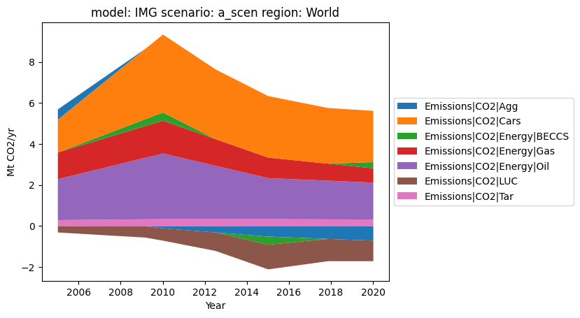
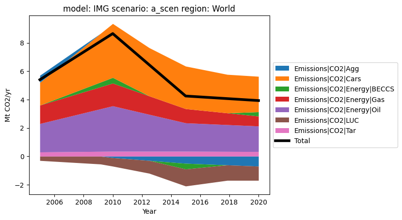
Pyam’s stackplot method plots the stacks in the clearest way possible, even when some emissions are negative. The optional total keyword arguments also allows the user to include a total line on their plot.
[3]:
df.plot.stack()
[3]:
<Axes: title={'center': 'model: IMG scenario: a_scen region: World'}, xlabel='Year', ylabel='Mt CO2/yr'>
[4]:
df.plot.stack(total=True)
[4]:
<Axes: title={'center': 'model: IMG scenario: a_scen region: World'}, xlabel='Year', ylabel='Mt CO2/yr'>
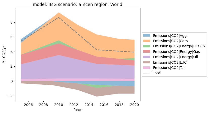
The appearance of the stackplot can be simply controlled via kwargs. The appearance of the total line is controlled by passing a dictionary to the total_kwargs keyword argument.
[5]:
df.plot.stack(alpha=0.5, total={"color": "grey", "ls": "--", "lw": 2.0})
[5]:
<Axes: title={'center': 'model: IMG scenario: a_scen region: World'}, xlabel='Year', ylabel='Mt CO2/yr'>
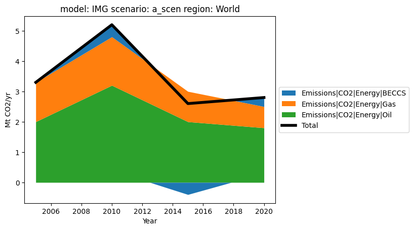
If the user wishes, they can firstly filter their data before plotting.
[6]:
df.filter(variable="Emissions|CO2|Energy*").plot.stack(total=True)
[6]:
<Axes: title={'center': 'model: IMG scenario: a_scen region: World'}, xlabel='Year', ylabel='Mt CO2/yr'>
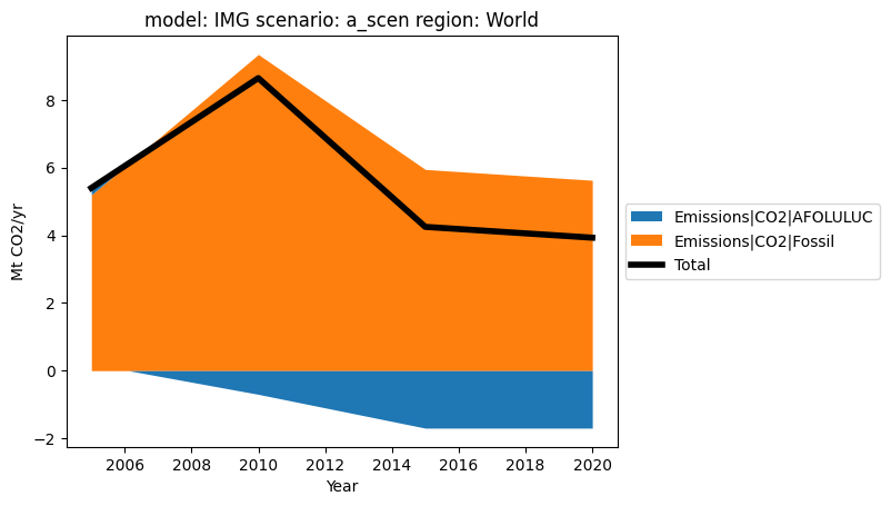
Using aggregate, it is possible to create arbitrary sums of sub-sectors before plotting.
[7]:
pdf = df.copy()
afoluluc_vars = ["Emissions|CO2|LUC", "Emissions|CO2|Agg"]
fossil_vars = list(set(pdf.variable) - set(afoluluc_vars))
pdf.aggregate("Emissions|CO2|AFOLULUC", components=afoluluc_vars, append=True)
pdf.aggregate("Emissions|CO2|Fossil", components=fossil_vars, append=True)
pdf.filter(variable=["Emissions|CO2|AFOLULUC", "Emissions|CO2|Fossil"]).plot.stack(
    total=True
)
[7]:
<Axes: title={'center': 'model: IMG scenario: a_scen region: World'}, xlabel='Year', ylabel='Mt CO2/yr'>
Aggregating regions
Here we provide some sample data for the second part of this tutorial. This data is for a single model-scenario combination with a few subsectors of CO\(_2\) emissions. The emissions in the subsectors are both positive and negative and so provide a good test of the flexibility of our aggregation and plotting routines.
[8]:
df = IamDataFrame(
    pd.DataFrame(
        [
            [
                "IMG",
                "a_scen",
                "World",
                "Emissions|CO2",
                "Mt CO2/yr",
                4.6,
                5.3,
                5.5,
                4.3,
            ],
            [
                "IMG",
                "a_scen",
                "World",
                "Emissions|CO2|Fossil",
                "Mt CO2/yr",
                4.0,
                4.6,
                4.9,
                4.1,
            ],
            [
                "IMG",
                "a_scen",
                "World",
                "Emissions|CO2|AFOLU",
                "Mt CO2/yr",
                0.6,
                0.7,
                0.6,
                0.2,
            ],
            [
                "IMG",
                "a_scen",
                "World",
                "Emissions|CO2|Fossil|Energy",
                "Mt CO2/yr",
                3.6,
                4.1,
                4.3,
                3.6,
            ],
            [
                "IMG",
                "a_scen",
                "World",
                "Emissions|CO2|Fossil|Aviation",
                "Mt CO2/yr",
                0.4,
                0.5,
                0.6,
                0.5,
            ],
            [
                "IMG",
                "a_scen",
                "R5ASIA",
                "Emissions|CO2",
                "Mt CO2/yr",
                2.3,
                2.6,
                2.8,
                2.6,
            ],
            [
                "IMG",
                "a_scen",
                "R5ASIA",
                "Emissions|CO2|Fossil",
                "Mt CO2/yr",
                2.0,
                2.1,
                2.2,
                2.3,
            ],
            [
                "IMG",
                "a_scen",
                "R5ASIA",
                "Emissions|CO2|Fossil|Energy",
                "Mt CO2/yr",
                2.0,
                2.1,
                2.2,
                2.3,
            ],
            [
                "IMG",
                "a_scen",
                "R5ASIA",
                "Emissions|CO2|AFOLU",
                "Mt CO2/yr",
                0.3,
                0.5,
                0.6,
                0.3,
            ],
            [
                "IMG",
                "a_scen",
                "R5LAM",
                "Emissions|CO2",
                "Mt CO2/yr",
                1.9,
                2.2,
                2.1,
                1.2,
            ],
            [
                "IMG",
                "a_scen",
                "R5LAM",
                "Emissions|CO2|Fossil",
                "Mt CO2/yr",
                1.6,
                2.0,
                2.1,
                1.3,
            ],
            [
                "IMG",
                "a_scen",
                "R5LAM",
                "Emissions|CO2|Fossil|Energy",
                "Mt CO2/yr",
                1.6,
                2.0,
                2.1,
                1.3,
            ],
            [
                "IMG",
                "a_scen",
                "R5LAM",
                "Emissions|CO2|AFOLU",
                "Mt CO2/yr",
                0.3,
                0.2,
                0,
                -0.1,
            ],
        ],
        columns=[
            "model",
            "scenario",
            "region",
            "variable",
            "unit",
            2005,
            2010,
            2015,
            2020,
        ],
    )
)
df.head()
[8]:
| model | scenario | region | variable | unit | year | value | |
|---|---|---|---|---|---|---|---|
| 0 | IMG | a_scen | World | Emissions|CO2 | Mt CO2/yr | 2005 | 4.6 |
| 1 | IMG | a_scen | World | Emissions|CO2 | Mt CO2/yr | 2010 | 5.3 |
| 2 | IMG | a_scen | World | Emissions|CO2 | Mt CO2/yr | 2015 | 5.5 |
| 3 | IMG | a_scen | World | Emissions|CO2 | Mt CO2/yr | 2020 | 4.3 |
| 4 | IMG | a_scen | World | Emissions|CO2|Fossil | Mt CO2/yr | 2005 | 4.0 |
If we aggregate the regional values for a sector, we get back the world total.
[9]:
df.aggregate_region("Emissions|CO2|AFOLU")
[9]:
<class 'pyam.core.IamDataFrame'>
Index:
 * model    : IMG (1)
 * scenario : a_scen (1)
Timeseries data coordinates:
   region   : World (1)
   variable : Emissions|CO2|AFOLU (1)
   unit     : Mt CO2/yr (1)
   year     : 2005, 2010, 2015, 2020 (4)
[10]:
df.filter(variable="Emissions|CO2|AFOLU", region="World").timeseries()
[10]:
| 2005 | 2010 | 2015 | 2020 | |||||
|---|---|---|---|---|---|---|---|---|
| model | scenario | region | variable | unit | ||||
| IMG | a_scen | World | Emissions|CO2|AFOLU | Mt CO2/yr | 0.6 | 0.7 | 0.6 | 0.2 |
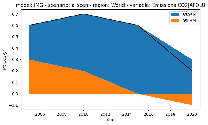
We can plot this as shown. The black line shows the World total (which is the same as the total lines shown in the previous part).
[11]:
import matplotlib.pyplot as plt

ax = plt.figure(figsize=(8, 4.5)).add_subplot(111)
df.filter(variable="Emissions|CO2|AFOLU").filter(region="World", keep=False).plot.stack(
    stack="region", ax=ax
)
df.filter(variable="Emissions|CO2|AFOLU", region="World").plot(ax=ax, color="black")
/home/docs/checkouts/readthedocs.org/user_builds/pyam-iamc/checkouts/latest/pyam/plotting.py:461: FutureWarning: The behavior of array concatenation with empty entries is deprecated. In a future version, this will no longer exclude empty items when determining the result dtype. To retain the old behavior, exclude the empty entries before the concat operation.
  _rows = pd.concat(
/home/docs/checkouts/readthedocs.org/user_builds/pyam-iamc/checkouts/latest/pyam/plotting.py:466: FutureWarning: The behavior of array concatenation with empty entries is deprecated. In a future version, this will no longer exclude empty items when determining the result dtype. To retain the old behavior, exclude the empty entries before the concat operation.
  pd.concat([_df, _rows.loc[_rows.index.difference(_df.index)]])
[11]:
<Axes: title={'center': 'model: IMG - scenario: a_scen - region: World - variable: Emissions|CO2|AFOLU'}, xlabel='Year', ylabel='Mt CO2/yr'>
Even if there are sectors which are defined only at the world level (e.g. Emissions|CO2|Fossil|Aviation in our example), pyam will find them and include them when calculating the regional total if we specify components=True when using aggregate_region.
[12]:
df.aggregate_region("Emissions|CO2|Fossil", components=True).timeseries()
[12]:
| 2005 | 2010 | 2015 | 2020 | |||||
|---|---|---|---|---|---|---|---|---|
| model | scenario | region | variable | unit | ||||
| IMG | a_scen | World | Emissions|CO2|Fossil | Mt CO2/yr | 4.0 | 4.6 | 4.9 | 4.1 |
[13]:
df.filter(variable="Emissions|CO2|Fossil", region="World").timeseries()
[13]:
| 2005 | 2010 | 2015 | 2020 | |||||
|---|---|---|---|---|---|---|---|---|
| model | scenario | region | variable | unit | ||||
| IMG | a_scen | World | Emissions|CO2|Fossil | Mt CO2/yr | 4.0 | 4.6 | 4.9 | 4.1 |
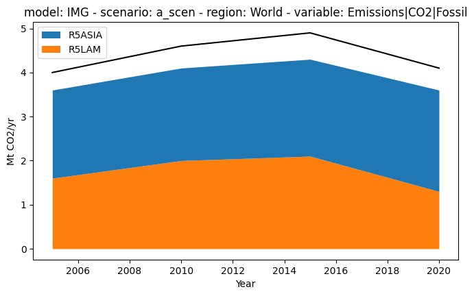
If we plot the regions vs. the total, in this case we will see a gap. This gap represents the emissions from variables only defined at the world level.
[14]:
ax = plt.figure(figsize=(8, 4.5)).add_subplot(111)
df.filter(variable="Emissions|CO2|Fossil").filter(
    region="World", keep=False
).plot.stack(stack="region", ax=ax)
df.filter(variable="Emissions|CO2|Fossil", region="World").plot(ax=ax, color="black")
/home/docs/checkouts/readthedocs.org/user_builds/pyam-iamc/checkouts/latest/pyam/plotting.py:466: FutureWarning: The behavior of array concatenation with empty entries is deprecated. In a future version, this will no longer exclude empty items when determining the result dtype. To retain the old behavior, exclude the empty entries before the concat operation.
  pd.concat([_df, _rows.loc[_rows.index.difference(_df.index)]])
[14]:
<Axes: title={'center': 'model: IMG - scenario: a_scen - region: World - variable: Emissions|CO2|Fossil'}, xlabel='Year', ylabel='Mt CO2/yr'>
We can verify this by making sure that adding the aviation emissions to the regional emissions does indeed give the aggregate total (a nicer way would be to plot these emissions in the stack above, pull requests which do so are welcome :D).
[15]:
import numpy as np

aviation_emms = df.filter(variable="*Aviation*").timeseries()
aggregate_emms = df.aggregate_region(
    "Emissions|CO2|Fossil", components=True
).timeseries()
aggregate_emms_region_only = (
    df.filter(region="World", keep=False)
    .aggregate_region("Emissions|CO2|Fossil")
    .timeseries()
)
np.isclose(
    aggregate_emms.values, aggregate_emms_region_only.values + aviation_emms.values
)
[15]:
array([[ True, True, True, True]])