Importing results from a GAMS model to an IamDataFrame
This tutorial illustrates how to extract results from any GAMS model (via the gdx file) and cast them to an IamDataFrame for further processing.
![]()
The workflow presented here uses the GAMS Python API (read the docs) and the gamstransfer module.
Follow these steps to install the requirements:
Manually install the GAMS API, follow one of the options in this description.
TL;DR: search for the folder “api_38” in the GAMS installation folder on your machine and run
python setup.py install
Install the schema package via
pip install schema
This is a dependency of the gamstransfer module.
This notebook was run with Python 3.8 and GAMS 33.2 on Mac OS.
The transport model
The model used for this illustration is the transport model by Rosenthal, frequently used for tutorials and examples.
The complete model is repeated here for clarity - note the last line which exports the results to a file in the GAMS Data Exchange (gdx) format.
*Basic example of transport model from GAMS model library

$Title  A Transportation Problem (TRNSPORT,SEQ=1)
$Ontext

This problem finds a least cost shipping schedule that meets
requirements at markets and supplies at factories.

Dantzig, G B, Chapter 3.3. In Linear Programming and Extensions.
Princeton University Press, Princeton, New Jersey, 1963.

This formulation is described in detail in:
Rosenthal, R E, Chapter 2: A GAMS Tutorial. In GAMS: A User's Guide.
The Scientific Press, Redwood City, California, 1988.

$Offtext

Sets
     i   canning plants   / seattle, san-diego /
     j   markets          / new-york, chicago, topeka / ;
Parameters
     a(i)  capacity of plant i in cases
       /    seattle     350
            san-diego   600  /
     b(j)  demand at market j in cases
       /    new-york    325
            chicago     300
            topeka      275  / ;
Table d(i,j)  distance in thousands of miles
                  new-york       chicago      topeka
    seattle          2.5           1.7          1.8
    san-diego        2.5           1.8          1.4  ;
Scalar f  freight in dollars per case per thousand miles  /90/ ;
Parameter c(i,j)  transport cost in thousands of dollars per case ;
          c(i,j) = f * d(i,j) / 1000 ;
Variables
     x(i,j)  shipment quantities in cases
     z       total transportation costs in thousands of dollars ;

Positive Variable x ;

Equations
     cost        define objective function
     supply(i)   observe supply limit at plant i
     demand(j)   satisfy demand at market j ;

cost ..        z  =e=  sum((i,j), c(i,j)*x(i,j)) ;

supply(i) ..   sum(j, x(i,j))  =l=  a(i) ;

demand(j) ..   sum(i, x(i,j))  =g=  b(j) ;

Model transport /all/ ;

Solve transport using lp minimizing z ;

Display x.l, x.m ;

Execute_unload 'transport_tutorial.gdx';
Import results from the gdx file
The first cell imports pyam and the two GAMS packages used in this tutorial.
[2]:
from gams import GamsWorkspace
from gamstransfer import GdxContainer

gdx = GdxContainer(GamsWorkspace().system_directory, "transport_tutorial.gdx")
gdx.rgdx()
Cast results to an IamDataFrame
The first cell in this section defines the model and scenario identifiers, which are identical for all results.
[3]:
args = dict(model="transport", scenario="baseline")
The objective value
The first cell in this section reads the value of the objective function, adds the year and displays the data.
cost.The last cell displays the data of the IamDataFrame.
[4]:
z = gdx.to_dataframe("z")["elements"]
z["year"] = 2020
z
[4]:
| L | year | |
|---|---|---|
| 0 | 153.675 | 2020 |
[5]:
from pyam import IamDataFrame

df = IamDataFrame(z, variable="cost", region="USA", unit="$", value="L", **args)
[6]:
df.timeseries()
[6]:
| 2020 | |||||
|---|---|---|---|---|---|
| model | scenario | region | variable | unit | |
| transport | baseline | USA | cost | $ | 153.675 |
Optimal shipment of quantities
x.L) is read by default by the GdxContainer.to_dataframe() function.[7]:
x = gdx.to_dataframe("x")["elements"]
x["year"] = 2020
x
[7]:
| i | j | L | year | |
|---|---|---|---|---|
| 0 | seattle | new-york | 50.0 | 2020 |
| 1 | seattle | chicago | 300.0 | 2020 |
| 2 | seattle | topeka | 0.0 | 2020 |
| 3 | san-diego | new-york | 275.0 | 2020 |
| 4 | san-diego | chicago | 0.0 | 2020 |
| 5 | san-diego | topeka | 275.0 | 2020 |
There are several ways to coerce the “from-to” dimension of the mathematical formulation to the “variable/region” format used in the IAMC data standard. In this example, we define a variable supply|* where * is the supply location and we use the demand center as the region.
This is implemented by adding a column ‘type’ to the shipment-dataframe and appending a new object to the results IamDataFrame concatening the ‘type’ column and the origin column ‘i’.
[8]:
x["type"] = "supply"
[9]:
df.append(
    x, variable=["type", "i"], value="L", region="j", unit="cases", **args, inplace=True
)
Market prices at the demand centers
The market price can be determined from the marginal value (field: M) of the demand-constraint equations.
[10]:
demand = gdx.to_dataframe("demand", fields="M")["elements"]
demand["year"] = 2020
demand
[10]:
| j | M | year | |
|---|---|---|---|
| 0 | new-york | 0.225 | 2020 |
| 1 | chicago | 0.153 | 2020 |
| 2 | topeka | 0.126 | 2020 |
[11]:
df.append(
    demand,
    variable="market price",
    value="M",
    region="j",
    unit="$/case",
    **args,
    inplace=True,
)
[12]:
df.timeseries()
[12]:
| 2020 | |||||
|---|---|---|---|---|---|
| model | scenario | region | variable | unit | |
| transport | baseline | USA | cost | $ | 153.675 |
| chicago | market price | $/case | 0.153 | ||
| supply|san-diego | cases | 0.000 | |||
| supply|seattle | cases | 300.000 | |||
| new-york | market price | $/case | 0.225 | ||
| supply|san-diego | cases | 275.000 | |||
| supply|seattle | cases | 50.000 | |||
| topeka | market price | $/case | 0.126 | ||
| supply|san-diego | cases | 275.000 | |||
| supply|seattle | cases | 0.000 |
Postprocessing to compute aggregate results
It is often practical to not only have results at the most disaggregated level, but to also add aggregated results to the output. The pyam package offers several utilities to perform aggregation or validation; the following cell computes the total supply to each demand city and appends it to the IamDataFrame.
The second cell again displays the complete data to illustrate the aggregation feature.
[13]:
df.aggregate("supply", append=True)
[14]:
df.timeseries()
[14]:
| 2020 | |||||
|---|---|---|---|---|---|
| model | scenario | region | variable | unit | |
| transport | baseline | USA | cost | $ | 153.675 |
| chicago | market price | $/case | 0.153 | ||
| supply | cases | 300.000 | |||
| supply|san-diego | cases | 0.000 | |||
| supply|seattle | cases | 300.000 | |||
| new-york | market price | $/case | 0.225 | ||
| supply | cases | 325.000 | |||
| supply|san-diego | cases | 275.000 | |||
| supply|seattle | cases | 50.000 | |||
| topeka | market price | $/case | 0.126 | ||
| supply | cases | 275.000 | |||
| supply|san-diego | cases | 275.000 | |||
| supply|seattle | cases | 0.000 |
Visualization of results
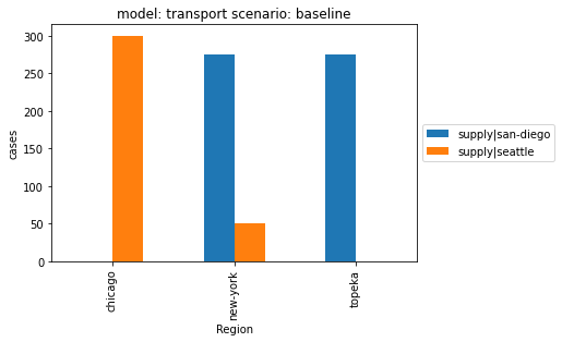
The pyam package includes a powerful plotting and visualization library. Most features are geared for timeseries data (for plotting development over time), but some are useful even for this small, stylized application: the next cell shows the regional share of supply from the two supply locations to the three demand centers.
[15]:
df.filter(variable="supply|*").plot.bar(x="region")
[15]:
<AxesSubplot:title={'center':'model: transport scenario: baseline'}, xlabel='Region', ylabel='cases'>
Visit the pyam plotting gallery for more features and options!
Exporting to different file formats
You can use pyam to export the processed data in the IAMC format as an Excel table.
[16]:
df.to_excel("transport.xlsx")
pyam also supports export to different file formats, for example the frictionless data package!
[17]:
df.to_datapackage("transport.zip")
[17]:
<datapackage.package.Package at 0x7fd68e73d970>
Questions? Take a look at this tutorial for first steps with pyam - then join our mailing list!